
Analyse your data as you go, and stop just in time
…to confirm an election was counted correctly
Damjan Vukcevic
Statistics seminar, University of Sydney
17 April 2026
Overview
Analyse and stop when you like…

Overview
- Sequential analysis
- Auditing preferential elections
Will not cover
- E-statistics (e-values, e-processes)
Sequential analysis
Sequential probability ratio test (SPRT)

Developed by Wald (1945)
Birth of sequential analysis
Binary data example
Data (X_i): 0, 0, 1, 1, 0, 1, \dots
Hypotheses: \begin{cases} H_0\colon p = p_0 \\ H_1\colon p = p_1 \end{cases}

Binary data example
Test statistic: S_t = \frac{L_t(p_1)}{L_t(p_0)} = \frac{\Pr(X_1, \dots, X_t \mid H_1)} {\Pr(X_1, \dots, X_t \mid H_0)} = \frac{p_1^{Y_t} (1 - p_1)^{t - Y_t}} {p_0^{Y_t} (1 - p_0)^{t - Y_t}}
Where: Y_t = \sum_{i=1}^t X_i
Binary data example

Binary data example
Stopping rule: \begin{cases} S_t \leqslant \frac{\beta}{1 - \alpha} & \Rightarrow \text{accept } H_0 \\ S_t \geqslant \frac{1 - \beta}{\alpha} & \Rightarrow \text{accept } H_1 \\ \text{otherwise} & \Rightarrow \text{keep sampling} \end{cases}
Error control:
- Type 1 error \leqslant \alpha
- Type 2 error \leqslant \beta
Binary data example

Sample size distribution
Parameters:
- p_0 = 0.5
- p_1 = 0.7 = p
- \alpha = \beta = 0.1
n = 38 for fixed-n test with same power
SPRT often stops earlier
Benefits 👍
- Safe: can “peek” 👁️ at the data
- Efficient: small sample sizes
- Can “accept” H_0
- Principled “no decision” is possible
Disadvantages 👎
- Operational planning more complex
- Sample size unknown in advance
- Sample size could be very large
- Only simple vs simple (for now…)
SPRT in general
H_0\colon X \sim f_0(\cdot) \quad \text{vs} \quad H_1\colon X \sim f_1(\cdot)
Test statistic: S_t = \frac{f_1(X_1, X_2, \dots, X_t)} {f_0(X_1, X_2, \dots, X_t)}
Test statistic, with iid observations: S_t = \prod_{i=1}^t \frac{f_1(X_i)}{f_0(X_i)} = S_{t - 1} \times \frac{f_1(X_t)}{f_0(X_t)}
“Tests of power one”
- Set \beta = 0
- Stopping rule:
Reject H_0 once S_t \geqslant 1 / \alpha - Never “accept” H_0
- No type II error (power = 1), but might have n = \infty.

Why is the SPRT “safe”?
Martingale

“Stays the same” on average
Supermartingale 🦸

“Stays the same or reduces in value” on average
(Super)martingales
Martingale condition: \mathbb{E}\left(S_{t+1} \mid X_1, \dots, X_t\right) = S_t
Supermartingale condition: \mathbb{E}\left(S_{t+1} \mid X_1, \dots, X_t\right) \leqslant S_t
Ville’s inequality
Let S_0, S_1, S_2, \dots be a test supermartingale (TSM):
has non-negative terms (S_i \geqslant 0) and starting value S_0 = 1.
For any \alpha > 0, \Pr\left(\max_t (S_t) \geqslant \frac{1}{\alpha}\right) \leqslant \alpha
Tests based on martingales
- S_t should be a test supermartingale (TSM) under H_0
- S_t should grow quickly under H_1


Tests based on martingales
Decision rule:
- Reject H_0 if S_t \geqslant 1 / \alpha
- Otherwise keep sampling (or give up)
Ville’s inequality \Rightarrow anytime-valid type I error control
Growth rate under H_1 \rightarrow statistical efficiency (“power”)
The SPRT is a martingale
At time t: \mathbb{E}_{H_0} \left(\frac{f_1(X_t)}{f_0(X_t)}\right) = \int \frac{f_1(x)}{f_0(x)} f_0(x) \, dx = \int f_1(x) \, dx = 1
This implies the martingale condition.
Beyond simple hypotheses
H_0\colon \theta = \theta_0 \quad \text{vs} \quad H_1\colon \theta \in \mathcal{A}
Plug-in strategy: S_t = S_{t-1} \times \frac{f(X_t \mid \hat\theta_t)}{f(X_t \mid \theta_0)} \hat\theta_t = a(X_1, X_2, \dots, X_{t-1}) \in \mathcal{A}
Beyond simple hypotheses
H_0\colon \theta = \theta_0 \quad \text{vs} \quad H_1\colon \theta \in \mathcal{A}
Mixture strategy: S_t = S_{t-1} \times \frac{\int_{\mathcal{A}} f(X_t \mid \theta) \, g_t(\theta) \, d\theta}{f(X_t \mid \theta_0)} g_t(\theta) \text{ is a distribution over } \mathcal{A} g_t(\theta) \text{ can depend on } X_1, X_2, \dots, X_{t-1}
Further reading
“Safe anytime-valid inference” (SAVI)
Auditing preferential elections
Acknowledgements 💟
- Michelle Blom
- Alexander Ek
- Floyd Everest
- Dania Freidgeim
- Dennis Leung
- Philip Stark
- Peter Stuckey
- Vanessa Teague
Australian Research Council:
- Discovery Project DP22010101
- OPTIMA ITTC IC200100009
Counting the votes

Counting the votes

Counting the votes

What can go wrong?
- Human error
- Machine malfunction
- Malicious interference
More automation \rightarrow less scrutiny
Election audits
Goal:
- Detect (and correct) wrong election outcomes
How: statistics! 📊
- Sample the ballot papers
- Infer the winners
- Use sequential tests
Two-candidate example
Election: Albo vs Dutton 🤼
p = \text{Proportion of votes for Albo}
\begin{cases} H_0\colon p \leqslant 0.5, & \text{Albo did not win} \\ H_1\colon p > 0.5, & \text{Albo won} \end{cases}
Two-candidate example
SPRT with a plug-in estimator of p:
S_t = S_{t-1} \times \frac{\Pr(X_t \mid \hat{p}_t)}{\Pr(X_t \mid p = 0.5)} \hat{p}_t = h(X_1, \dots, X_{t-1}) \in (0.5, 1]
“ALPHA supermartingale” (Stark 2023)
Preferential elections

Voting
Rank the candidates in order of preference.
Examples
- (1) Garth, (2) Michael, (3) Wei
- (1) Michael, (2) Garth, (3) Wei
- (1) Wei, (2) Garth
- (1) Michael
Counting the votes
Iterative algorithm:
- Eliminate least preferred candidate; redistribute their votes
- Last candidate standing is the winner.
This produces an elimination order.
Example
[Wei, Michael, Garth]
Garth is declared the winner
Auditing
H_0 = “someone else won the election”
H_0 includes all elimination orders with
alternative winners (“alt-orders”).
Example alt-orders
[Garth, Michael, Wei]
[Garth, Wei, Michael]
[Michael, Garth, Wei]
[Wei, Garth, Michael]
Auditing challenge
Need to reject every all-order
k candidates \Rightarrow \sim k! ballot types
k candidates \Rightarrow \sim k! alt-orders
Challenges
- High-dimensional parameter space
- Complex boundary between H_0 and H_1
Auditing strategy
- Decompose H_0 into simpler, 1-dimensional statements
- Test each statement separately
- Combine test results into a single decision
Null decomposition
Enumerate all alt-orders: 1, \dots, m
H_0^i = “alt-order i is true”
H_0 = H_0^1 \cup H_0^2 \cup \dots \cup H_0^m
Must reject every alt-order
Simple statements (“requirements”)
Example:
“Garth has more votes than Michael assuming that only
candidates in the set \mathcal{S} remain standing.”
Notation:
- DB(Garth > Michael, S)
Equivalent to a two-candidate election.
Can test using ALPHA.
Testing an alt-order
Alt-order: [Garth, Michael, Wei]
Requirements:
- DB(Michael > Garth, {G,M,W})
- DB(Wei > Garth, {G,M,W})
- DB(Wei > Michael, {M,W})
Alt-order is true \Leftrightarrow all of its requirements are true
Reject at least one requirement \Rightarrow reject the alt-order
Alt-orders as intersections
Alt-order i is an intersection of its requirements: H_0^i = R_i^1 \cap R_i^2 \cap \dots \cap R_i^{r_i}
Simpler, more generic notation: H = H^1 \cap H^2 \cap \dots \cap H^r
Adaptive weighting (for intersections)
Base TSM: for H^j
S_{j,t} = \prod_{i = 1}^t s_{j, i}
Intersection TSM: for H
S_t = \prod_{i = 1}^t \frac{\sum_j w_{j, i} \, s_{j, i}}{\sum_jw_{j, i}}
The weights w_{j, i} can depend on data up until time i - 1.
How to choose the weights w_{j, i}?
Weighting schemes
How to choose the weights w_{j, i}?
Ideas:
- Largest: Put weight 1 on the largest base TSM so far.
- Linear: Proportional to previous value, w_{j, i} = S_{j, i - 1}.
- Quadratic: Proportional to square of previous value, w_{j, i} = S_{j, i - 1}^2.
- Many more…
Compared about 30 schemes. “Largest” was often the best.
Weighting schemes

Scaling up
k! alt-orders
\rightarrow 💥 explosion of decompositions & intersections
Use combinatorial optimisation methods…
Suffix trees of partial alt-orders
graph TD
    A("[...1]")   --> B("[...2,1]")
    A("[...1]")   --> C("[...3,1]")
    A("[...1]")   --> D("[...4,1]")
    B("[...2,1]") --> E("[4,3,2,1]")
    B("[...2,1]") --> F("[3,4,2,1]")
    C("[...3,1]") --> G("[4,2,3,1]")
    C("[...3,1]") --> H("[2,4,3,1]")
    D("[...4,1]") --> I("[3,2,4,1]")
    D("[...4,1]") --> J("[2,3,4,1]")
Incremental expansion and pruning
graph TD
    A("[...1]")   --> B("[...2,1]")
    A("[...1]")   --> C("[...3,1]")
    A("[...1]")   --> D("[...4,1]")
    B("[...2,1]") --> E("[4,3,2,1]")
    B("[...2,1]") --> F("[3,4,2,1]")

style C fill:#fff0f5,stroke:#db7093,color:#db7093
style D fill:#fff0f5,stroke:#db7093,color:#db7093
Computational scale-up
‘Exhaustive’ implementation: up to 6 candidates
‘Incremental’ implementation: 55+ candidates
Summary
Sequential analysis allows for “safe” inference
Modern tools use TSMs (and e-processes)
Complex inference problems can be tackled sequentially with finite-sample guarantees.
Questions?
References 📚
Chugg, Ramdas, Grünwald (2026). E-values as statistical evidence: A comparison to Bayes factors, likelihoods, and p-values. arXiv:2603.24421.
Ek, Blom, Stark, Stuckey, Vukcevic (2024). Improving the Computational Efficiency of Adaptive Audits of IRV Elections. In: Electronic Voting. E-Vote-ID 2024. Lecture Notes in Computer Science 15014:37–53.
Ek, Stark, Stuckey, Vukcevic (2023). Adaptively Weighted Audits of Instant-Runoff Voting Elections: AWAIRE. In: Electronic Voting. E-Vote-ID 2023. Lecture Notes in Computer Science 14230:35–51.
Ramdas, Grünwald, Vovk, Shafer (2023). Game-Theoretic Statistics and Safe Anytime-Valid Inference. Statist. Sci. 38(4):576–601.
Stark (2023). ALPHA: Audit that learns from previously hand-audited ballots. Ann. Appl. Stat. 17(1):641–679.
Wald (1945). Sequential tests of statistical hypotheses. Ann. Math. Stat. 16(2):117–186.
Image sources 🖼️
The coin flipping graphic was designed by Wannapik.
The following photographs were provided by the Australian Electoral Commission and licensed under CC BY 3.0:
The Higgins ballot paper (available from The Conversation) was originally provided by Hshook/Wikimedia Commons and is licensed under CC BY-SA 4.0.
The photograph of Abraham Wald is freely available from Wikipedia.
The photograph of the 18th century print is freely available from the Digital Commonwealth; the original sits at the Boston Public Library.
Appendix
Binary data example


Martingales: origin

Martingales: origin
“Martingales”: 🎲 gambling strategies from 18th century France ♣️
These strategies cannot “beat the house”.
Martingales (in mathematics): represent the 💰 wealth over time of a gambler playing a fair game.
Betting analogy
Test statistic: S_t, a TSM under H_0
Intrepretation:
- S_t is the wealth of a gambler betting against H_0
- The gambler starts with $1
- They can vary their bets based on past data.
Gambler gets rich \rightarrow evidence against H_0
Ville’s inequality: “one in a million chance of becoming a millionaire”
E-variable
- A non-negative statistic E with: \mathbb{E}_{H_0}(E) \leqslant 1
- Betting analogy: payoff from a $1 bet in a (sub-)fair game
- Statistical interpretation: evidence against H_0
- Large E → strong evidence against H_0
- A realisation of E is an e-value.
Markov’s inequality
Let S be a non-negative random variable (S \geqslant 0).
For any \alpha > 0, \Pr\left(S \geqslant \frac{1}{\alpha}\right) \leqslant \alpha \cdot \mathbb{E}(S)
Let S = E, an e-variable. Under H_0 we have: \Pr\left(E \geqslant \frac{1}{\alpha}\right) \leqslant \alpha
Testing using e-values
Reject H_0 if E \geqslant 1 / \alpha
Markov’s inequality \Rightarrow type I error control
Note
- Alternative to using a p-value
- Generalises a likelihood ratio
Combining e-variables
A, B, C are e-variables
A, B, C independent \Rightarrow the product is an e-variable: E = A \cdot B \cdot C
The average is always an e-variable: E = \frac{A + B + C}{3}
(Easier than combining p-values!)
E-process
- Similar to a test supermartingale, but more general
- Sequence (E_t) with \mathbb{E}_{H_0}(E_\tau) \leqslant 1, \quad \text{for all stopping times } \tau.
- Connection with TSMs: E_t \leqslant \inf_{P \in H_0} S_t^{(P)}, \quad \text{where } S_t^{(P)} \text{ is a TSM for } P.
- Betting analogy: minimum wealth across simultaneous betting games
- Statistical interpretation: accumulated evidence against H_0
- Ville’s inequality applies
- Stop anytime → type I error control
Further reading
- E-values as statistical evidence
- Comparison with Bayes factors, likelihood ratios and p-values
P-values from e-values
P_t = \frac{1}{E_t}
E_t > \frac{1}{\alpha} \quad \Longleftrightarrow \quad P_t < \alpha
- P_t is an anytime-valid p-variable.
- A realisation of P_t is an anytime-valid p-value.
Confidence sequences
Fixed-sample hypothesis test \longleftrightarrow confidence interval (CI)
Sequential hypothesis test \longleftrightarrow confidence sequence (CS)


Don’t trust your scanner
Xerox bug 🐛:
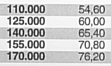
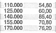
Source: https://www.dkriesel.com/
AWAIRE performance

“E-hacking”
Reanalysing the data with different test statistics (“betting strategies”) and only reporting the best one.
This is not safe stats.
Fundamental principle:
Declare your bet before you play.
Pre-registration is still an important tool.
However, anytime-valid methods retain flexibility even after pre-specification.
Research frontiers, in sequential analysis
- Improving efficiency (“power”)
- Complex, high-dimensional models
- Beyond iid/exchangeable data
- Connections with Bayesian approaches